A longer casino session changes more than the average loss

Set the finish line before calculating

The number of trials changes the distribution of a session result even when the house edge stays fixed. Expected loss grows with the number of equal stakes. The spread of cash results also grows, but at a different rate. Neither quantity, by itself, gives the probability of finishing ahead. We can calculate all three in a small teaching model and see where they disagree.

This is useful when an online-casino discussion turns a long-run percentage into a claim about tonight's result. The experiment below describes no commercial game. It has two outcomes, a fixed £1 stake, a specified finish after a set number of independent trials, and enough notional funds to complete every trial. We do not model deposits, bonuses, interrupted play or a balance running out.

That last condition matters. A session that ends after ten trials and a session that ends whenever its available balance is exhausted are different experiments. So is a session stopped at the first profit. Changing the stopping instruction after calculating the answer changes the question. Write the instruction down first, including whether finishing exactly level counts as success.

Give every trial a cash result

Our hypothetical trial pays £2 back, including the £1 stake, with probability 0.49. Otherwise it returns nothing. The net result is therefore plus £1 or minus £1. Those are teaching assumptions, not observed casino frequencies or an offer to play.

Expected net result per trial is (0.49 × £1) + (0.51 × −£1) = −£0.02. The expected loss is 2p for each £1 staked, which gives this model a 2% house edge. Expected gross return is £0.98. Notice that 98% is a ratio of expected money returned to money staked; the probability of the positive outcome is 49%.

For n trials, let K be the number of positive outcomes. There are n − K negative outcomes. The final net result in pounds is K − (n − K), or 2K − n. That short expression accounts for every stake, including the losing ones. Counting only the £2 prizes would leave out the total cost and would answer a gross-return question instead.

The Commission's public RTP explanation likewise distinguishes an average from an individual session. Its machine-specific averaging examples are not the trial counts used here. Our numbers come from the explicitly defined experiment.

Calculate the whole distribution

With a constant probability and independent trials, K follows a binomial distribution. NIST gives the probability of k successes as C(n,k) × p^k × (1−p)^(n−k). Here p is 0.49, and C(n,k) counts how many different sequences contain that many positive outcomes. The ordering changes the route, but not the final value of 2K − n.

Finishing ahead means 2K − n > 0. For ten trials that requires at least six positive outcomes. For 100 it requires at least 51, and for 1,000 at least 501. Add the binomial probabilities from that threshold through n to obtain the chance of a positive final result. Exactly half positive outcomes produces a tie for these even trial counts.

For example, the probability of a tie after ten trials is C(10,5) × 0.49^5 × 0.51^5, approximately 24.56%. Six through ten positive outcomes together have probability 35.26%. The remaining 40.18% finishes below the starting amount. These three mutually exclusive outcomes total 100%, apart from rounding. No simulated sample or selection of lucky paths is involved.

Compare three fixed endpoints

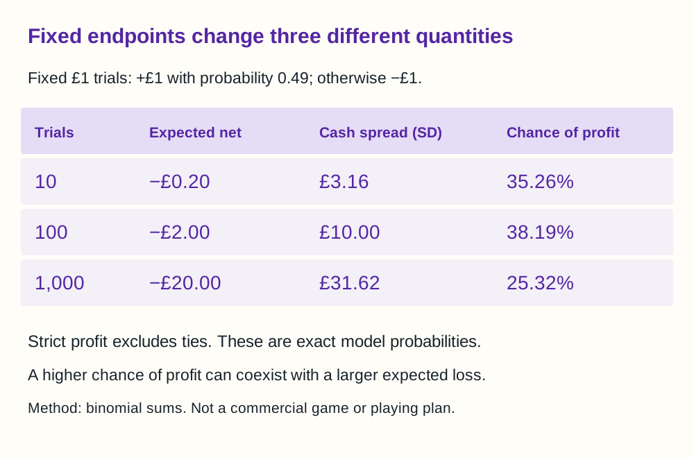
After ten trials the expected net result is −£0.20, the standard deviation of the final cash result is £3.16, and the probability of finishing ahead is 35.26%. After 100 trials those figures are −£2.00, £10.00 and 38.19%. After 1,000 they are −£20.00, £31.62 and 25.32%. All percentages are exact binomial sums rounded to two decimal places; cash spread is rounded in the same way.

The middle row is deliberately awkward. In this model, moving from ten to 100 trials increases the chance of finishing strictly ahead even though the expected loss becomes larger. The tie probability falls from 24.56% to 7.80%; the probability mass is distributed across different final results. A claim that every increase in session length must reduce the chance of a positive result would therefore be false.

That observation is not a reason to choose 100 trials. It shows why the chance of any profit is an incomplete financial description. It says nothing about how large the positive and negative results are. The negative expectation remains, and the cash spread is wider. A single percentage cannot rank these experiments on behalf of a person's finances or wellbeing.

Cash variation and percentage variation move differently

NIST gives the standard deviation of K as √[np(1−p)]. Since our net result is 2K − n, its standard deviation is 2√[n × 0.49 × 0.51] pounds. The subtraction moves the centre without changing the spread; multiplying by two doubles the spread. This produces the £3.16, £10.00 and £31.62 figures above.

Divide those spreads by total stakes of £10, £100 and £1,000. The corresponding percentages are approximately 31.62%, 10.00% and 3.16%. The result becomes less variable relative to turnover while remaining more variable in pounds. These are compatible statements with different denominators.

Standard deviation is a measure of spread, not a maximum loss, a promised range or a personal budget. We have not claimed that a specified proportion of outcomes lies within one standard deviation. Such a statement would require examining this distribution rather than borrowing a normal-distribution slogan.

Nor is turnover the same thing as fresh money deposited. Reusing a returned stake creates another stake in the arithmetic. The model records each trial's cost and result; it does not infer a required deposit from total turnover.

An endpoint is not the journey to it

Consider two invented four-trial paths: positive, positive, negative, negative; and negative, negative, positive, positive. Both finish level under our settlement rule. The first passes through a £2 gain, the second through a £2 loss. A final-result distribution treats their endpoint identically, although a limited starting balance could make the second route impossible to finish.

Our binomial calculation consequently cannot answer the chance of running out of money before trial 100. That is a path question requiring a starting balance and a rule for what happens when the next stake is unavailable. It also cannot tell you the largest loss encountered along the way. Recording the endpoint discards that information.

This distinction matters when reading screenshots of online-casino balances. A selected final balance does not identify the initial balance, intervening deposits, stakes, withdrawals or stopping rule. Even an authentic screenshot may provide insufficient information for the proposed calculation. Our result is reproducible because the missing ingredients have been specified in advance, not because the model resembles every real session.

Check whether the assumptions survive contact with the game

The Gambling Commission's RTS 7 sets requirements for random outcomes in covered remote products and prohibits compensated adaptive behaviour. It also recognises changes specified by game rules, including bonus rounds and progressive jackpots. A regulatory requirement is not our own test of a particular operator or proof that every commercial game fits a two-outcome binomial model.

Multiple prize sizes would require more than a count of positive outcomes. Changing stakes would require accounting for each stake. Sampling without replacement may change conditional probabilities. A rules-defined state change may alter which probability applies. These are reasons to examine the specification before choosing a formula.

The teaching model keeps these complications out so that one question stays visible: what changes when only the fixed endpoint changes? If a real product's full probabilities are unavailable, do not insert its advertised RTP as p. RTP is a monetary expectation, and p here is the probability of one precisely defined outcome. That substitution would generate precise-looking answers about an experiment nobody described.

Read a session claim in four fields

A useful mathematical note records the outcome definition, the stopping rule, the unit and the assumptions. For this experiment: finish strictly ahead; stop after n trials; measure net pounds and probability separately; assume independent identical £1 trials with the stated two-outcome settlement.

Now keep the three outputs beside one another. Expected loss gives the average net cost across the model's possibilities. Standard deviation describes how dispersed the cash results are. Probability of profit counts outcomes above zero without weighing how large those profits are. A tie remains a separate result.

The worked comparison is a way to inspect a claim, not to optimise a gambling session. It gives no recommended duration, stake or recovery plan. A larger chance of a small positive endpoint can coexist with a worse average result. More trials do not remove the possibility of losses or make the next outcome compensate for the last one. Choosing not to play requires no probability calculation.